Content Classification of Multimedia Documents using Partitions of Low-Level Features
First presented at the International Conference
on Content-Based Multimedia Indexing 2003,
extended and revised for JVRB
urn:nbn:de:0009-6-7607
Abstract
Audio-visual documents obtained from German TV news are classified according to the IPTC topic categorization scheme. To this end usual text classification techniques are adapted to speech, video, and non-speech audio. For each of the three modalities word analogues are generated: sequences of syllables for speech, “video words” based on low level color features (color moments, color correlogram and color wavelet), and “audio words” based on low-level spectral features (spectral envelope and spectral flatness) for non-speech audio. Such audio and video words provide a means to represent the different modalities in a uniform way. The frequencies of the word analogues represent audio-visual documents: the standard bag-of-words approach. Support vector machines are used for supervised classification in a 1 vs. n setting. Classification based on speech outperforms all other single modalities. Combining speech with non-speech audio improves classification. Classification is further improved by supplementing speech and non-speech audio with video words. Optimal F-scores range between 62% and 94% corresponding to 50% - 84% above chance. The optimal combination of modalities depends on the category to be recognized. The construction of audio and video words from low-level features provide a good basis for the integration of speech, non-speech audio and video.
Keywords: Audio-visual content classification, support vector machines, speech recognition, integration of modalities
Subjects: Support Vector Machines, Content Analysis, Automatic Speech Recognition
Content processing of speech, non-speech audio and video data is one of the central issues of recent research in information management. During the last years new methods for the classification of text, audio, video and voice information have been developed, but Multimodal analysis and retrieval algorithms especially towards exploiting the synergy between the various media is still considered as one of the major challenges of future research in multimedia information retrieval [ LSDJ06 ]. The combination of features from different modalities should lead to an improvement of results. We present an approach to supervised multimedia classification that allows to benefit from the joint exploitation of speech, video and non-speech audio.
We use low-level features such as color correlograms, spectral flatness, and syllable sequences for the integrated classification of audio-visual documents. The novelty of our approach is to process non-speech information in such a way that it can be represented jointly with linguistic information in a generalised term-frequency vector. This allows for subsequent processing by usual text-mining techniques including text classification, semantic spaces, and topic-maps.
Support Vector Machines (SVM) have been applied successfully to text classification tasks [ Joa98, DPHS98, DWV99, LK02 ]. We adapt common SVM text classification techniques to audio-visual documents which contain speech, video, and non-speech audio data. To represent these documents we apply the bag-of-words approach which is common to text classification. We generate word analogues for the three modalities: sequences of phonemes or syllables for speech, “video-words” based on low level color features for video, and “audio-words” based on low-level spectral features for general audio.
We assume that there is a hidden code of audio-visual communication. This code cannot be made explicit, it consists of a tacit knowledge that is shared and used by the individuals of a communicating society. Furthermore we assume that, for the purpose of subsequent classification, the unknown hidden code can be substituted by an arbitrary partition of the feature space. Our approach is inspired by the fenone recognition technique which is an alternative to standard speech recognition for classification purposes. Fenone recognition has been done successfully by Harbeck [ Har01 ] for the speech domain. Instead of using a standard speech recognizer, which recognises phonemes — i.e. areas in the feature space that are defined by linguistic tradition — a cluster analysis is performed, which segments the feature space in a data driven fashion. The recognized fenones serve as analogues to phonemes and are forwarded to a subsequent classification procedure. The advantage of fenones over phonemes is that they can be calculated even if there is no a priory knowledge of the language and consequently of the code under consideration. Their disadvantage is that they do not accommodate human interpretation.
Thus as proposed by [ Leo02 ] each element of a partition,i.e. a disjoint segmentation, of the feature space can be considered as a unit — sign — of the audio-visual code whereas the partition itself is the respective vocabulary of audio or video-signs. The visual vocabularies that we create are not sets of elementary symbols, but abstract subsets of the feature space, which is defined by the attribute values of visual low-level features. They have nothing in common with visual vocabularies that have been used elsewhere [ FGJ95 ] for visual programming purposes. Instead they resemble to what is called a mood chart in the area of visual design [ RPW06 ].
The reason for using an automatically generated vocabulary inducing a set of artificial (and therefore inexplicable) concepts is that detecting a wider set of concepts other than human faces in images or video scenes turned out to be fairly difficult. Lew [ Lew00 ] showed a system for detecting sky, trees, mountains, grass, and faces in images with complex backgrounds. Fan, et al. [ FGL04 ] used multi-level annotation of natural scenes using dominant image components and semantic concepts. Li and Wang [ LW03 ] used a statistical modeling approach in order to convert images into keywords. Rautiainen, et al. [ RSP03 ] used temporal gradients and audio analysis in video to detect semantic concepts.
The non-speech audio vocabularies that we create are not a set of elementary motifs of harmonic stereotypes, but abstract subsets of the feature space, which is defined by the attribute values of acoustic low-level features. Our corpus of audio-visual documents consists of news recordings which contain very few segments that could be called musical in a narrower sense. Therefore automatic music transcription as for example in [ CLL99 ] is not appropriate for our material.
One further reason for the application of non-speech audio and video signs is that we want to take into account the entire document while preserving the essential information present in small temporal segments. Thus mapping short time intervals to video or audio signs as prototypical representations seems to be a promising approach for the representation of audio-visual scenes. Finally the application of audio and video signs is an integrated and successful approach to the fusion of speech, video and non-speech audio. We thus present a theoretical framework for the combination of audio and video information. This is currently considered as a challenging task [ LSDJ06 ].
In the next chapter we describe the corpus of audio-visual documents that was utilized for content classification. Feature extraction and the representation of audio-visual documents in the classifier′s input space is described in section 3. In section 4 we specify the classifier and its parameters. Results are presented in section 5 and in section 6 we conclude.
Table 1. Size of IPTC-classes in terms of number of documents. Only those classes, which contain more than 45 documents (left column) were considered.
|
Categories and number of documents |
|||
|
politics |
200 |
human interest |
40 |
|
justice |
120 |
disaster |
38 |
|
advertisement |
119 |
culture |
22 |
|
sports |
91 |
jingle |
22 |
|
conflicts |
85 |
health |
19 |
|
economy |
68 |
environmental issue |
17 |
|
labour |
49 |
leisure |
15 |
|
|
|
science |
13 |
|
|
|
education |
10 |
|
|
|
weather |
8 |
|
|
|
social issue |
6 |
|
|
|
religion |
4 |
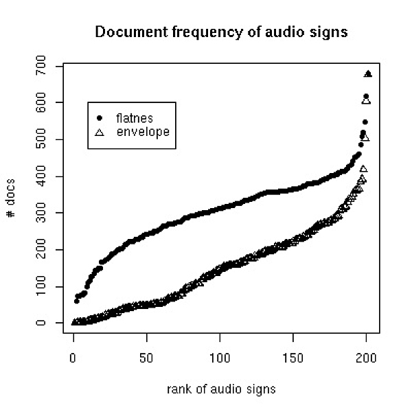
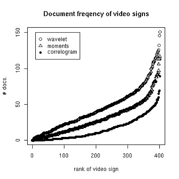
Figure 1. Rank distribution of document frequency of video and audio signs. The left panel shows the document frequency of the visual signs generated from the thee low level features described in section 3.2 . The right panel shows the document frequency for two audio features described in section 3.3 . Sizes of the visual and acoustic vocabulary are 400 and 200 signs respectively.
The data for the audio-visual corpus was obtained from two different German news broadcast stations: N24 and n-tv. The audio-visual stream was segmented manually into news items. This resulted in a corpus that consists of 693 audio-visual documents. Document length ranges between 30 sec. and 3 minutes. The semantic labeling of the news stories was done manually according to the categorization scheme of the International Press Telecommunications Council (IPTC) (see http://www.iptc.org). The material from N24 consists of 353 audio-visual documents and covers the period between May 15 and June 13, 2002 (including reports from the World Cup soccer tournament in Korea and Japan. This event can be considered as semantically unique. It does not appear in the training corpus for generating the audio-visual “vocabularies”, which were obtained from tv recordings of October 2002). The data from n-tv comprises 340 documents and covers the last seven days of April 2002. Table 1 shows the distribution of topic classes in the corpus. For convenience we added two classes “advertisement” and “jingle” to the 17 top level classes of the IPTC-categorization. The number of documents in the classes total more than 693. Some documents were attributed to two or three classes because of the ambiguity of their content. For example, audio-visual documents on the Israel-Palestine conflict often were categorized as belonging to both “politics” and “conflicts”.
The size of the classes in the audio-visual corpus varies considerably: “politics” comprises 200 audio-visual documents whereas “religion” contains just 4. We only used those seven categories with more than 45 documents (shown in the left column of table 1 ) for classification experiments. As will be described in section 4 we trained a separate binary classifier for each of these seven classes. All documents of the small categories (less than 45 documents) were always put in the set of counter-examples.
In Figure 1 the document frequency, i.e. the number of documents in which a given sign occurs, is calculated for different audio and video signs. Document frequency is a term weight that is commonly used in text mining applications in order to quantify how good a given term serves as an indicator of a document′s content. A term that occurs in all documents of a corpus is not considered as a useful indicator, whereas a term that occurs in few classes is supposed to be specific to the document′s content. It can be seen that most of the visual signs have a medium document frequency, which makes them useful for content classification. The non-speech audio signs show a less favourable pattern, rendering it inferior for content classification: most of the audio signs occur in more than a quarter of the documents. Some audio signs occur in nearly every document. As mentioned before the whole corpus comprises 693 documents.
In the same fashion as a speech recognizer has to be trained in order to acquire a model of the speech to be recognized, the vocabularies for video and non-speech audio have to be generated from a training corpus. In order to obtain significant results the training data has to be different from the data to be classified. Therefore the audio-visual corpus described above was not used for the generation of the visual and non-speech vocabulary, with the exception of some control experiments marked as “corpus” that are presented in figure 3 and 4 .
The feature extraction procedures for each of the three modalities speech, video and non-speech audio are independent from each other. As in [ PLL02 ] syllables are stringed together to form terms, that do not necessarily correspond to linguistic word boundaries. Video signs and non-speech audio signs are defined as subsets of the respective feature space. Sequences of video signs are referred to as video words, and sequences of non-speech audio signs are called audio words.
The automatic speech recognition system (ASR) was built using the ISIP (Institute for Signal and Information Processing) public domain speech recognition tool kit from Mississippi State University. We implemented a standard ASR system based on a Hidden Markov Model. The ASR used cross-word tri-phone models trained on seven hours of data recorded from radio documentary programs. These included both commentator speech and spontaneous speech in interviews, and were thus similar to speech occurring in TV news of our corpus.
The audio track of each audio-visual document was speaker segmented using the BIC algorithm [ TG99 ]. Breaks in the speech flow were located with a silence detector and the segments were cut at these points in order to insure that no segment be longer than 20 seconds. However, the acoustic signal was not separated into speech and non-speech segments. Therefore the output of the speech recognizer also consists of nonsense syllable sequences generated by the recognizer during music and other non-speech audio.
Table 2. Number of syllable-n-grams in the audio-visual corpus. The number of syllable-n-grams in the running text (tokens) as well as of different syllable-n-grams (types) are displayed.
|
Number of types (2nd line) and tokens (last line) of syllable n-grams |
|||||
|
n = 1 |
n = 2 |
n = 3 |
n = 4 |
n = 5 |
n = 6 |
|
3766 |
71505 |
153789 |
177478 |
182492 |
183707 |
|
189894 |
189212 |
188532 |
187853 |
187175 |
186497 |
The language model was trained on texts which were decomposed into syllables using the syllabification module of the BOSSII speech synthesis system [ SWH00 ]. Exploratory investigation allowed us to determine that 5000 syllables give good recognition performance. The syllable language model was a syllable tri-gram model and was trained on 64 million words from the German dpa newswire. The advantage of using a syllable-based language model instead of a word-based model is that words can be generated from syllables on-the-fly which leads to reduction of vocabulary size, less domain dependency and therefore less out-of-vocabulary errors. A syllable base language model is especially useful when the ASR is applied to a language which is highly productive at the morpho-syntactic level, like German in our case [ LEP02 ].
From the recognized syllables, n-grams (1 ≤ n ≤ 6) were constructed in order to reach a level of semantic specificity comparable to that of words. The use of n-grams also makes it possible to adjust the linguistic units appropriate to the trade-off between semantic specificity and low probability of occurrence, which is especially important when document classes are small. From previous experiments on textual data we have observed that unit size is among the most important determinants of the classification accuracy of support vector machines [ PLL02 ].
As the number of syllable n-grams in the audio-visual documents is large, a statistical test is used to eliminate unimportant ones. First it is required that each term must occur at least twice in the corpus. In addition, the hypothesis that there is a statistical relation between the document class under consideration and the occurrence of a term is investigated by a χ²-statistic. A term is rejected when its χ² statistic is below a threshold θ. The values of θ used in the experiments are θ = 0.1 and θ = 1.
In the same way as a speech recognizer has to be trained in order to learn a vocabulary of phonemes (acoustic model) and how they are combined to form syllables or words (language model), a visual vocabulary has to be learned from training data. The generation of such a visual vocabulary was done on a training corpus of video data from recorded TV news broadcasts. This training corpus is different from the corpus described in the preceding section. It contains 11 hours of video sampled in October 2002.
First the video data was split into individual frames. To reduce the huge amount of frames, only one frame per second of video material was selected. This could be done because the similarity between neighbouring frames is usually high. In this manner the frame count was reduced by approximately a factor 3. After that, the three low-level features were extracted from the reduced set of frames and the buoy generation method [ Vol02 ] was applied to their respective feature spaces, generating a disjoint segmentation. In this way sets of prototypical images were obtained for each of the three features. These sets are the visual vocabularies and their elements are the video signs. Visual vocabularies of the size of 100, 200, 400 and 800 video signs were created.
Table 3. The number of running words (tokens) and of different video words (types) is displayed for a vocabulary size of 400 video signs based on different features, A: moments of 29 colors, B: correlogram of 9 colors, C: wavelet of 9 colors
|
Number video sign n-grams in the AV-corpus |
|||||||
|
|
|
n = 1 |
n = 2 |
n = 3 |
n = 4 |
n = 5 |
n = 6 |
|
A |
types |
363 |
5305 |
6947 |
6749 |
6380 |
5967 |
|
tokens |
9060 |
8378 |
7696 |
7128 |
6617 |
6128 |
|
|
B |
types |
363 |
5495 |
7005 |
6793 |
6421 |
6005 |
|
tokens |
9060 |
8378 |
7696 |
7128 |
6617 |
6128 |
|
|
C |
types |
298 |
5050 |
6909 |
6789 |
6416 |
5997 |
|
tokens |
9060 |
8378 |
7696 |
7128 |
6617 |
6128 |
|
To represent the video scenes of the audio-visual corpus the video stream is first segmented into coherent units (shots). Then for each shot a representative image is selected, which is called the key frame of the shot. The segmentation is done by algorithms monitoring the change of image over time. Two adjacent frames are compared and their difference is calculated. The differences are summed, and when the sum exceeds a given threshold a shot-boundary is detected, and the key frame of the shot is calculated. For each shot there are three low-level features, which are extracted from its key frame: first and second moments of 29 colors, a correlogram calculated on the basis of 9 major colors, and a wavelet that was also based on 9 major colors. These features where chosen because they combine aspects of color and texture. Each of the three visual features is mapped to the nearest video-sign in the respective visual vocabulary. From the video signs, n-grams (1 ≤ n ≤ 6) were generated by stringing video signs together according to their sequence in the audio-visual corpus. These n-grams are also referred to as “video words”.
As mentioned above, the results presented in the paper were obtained by using visual vocabularies that were generated from a training corpus of 11 hours of video in October 2002. Note that the audio-visual corpus to be classified was sampled three to six months before the training corpus, in the period between April and June 2002 (see section 2 ). In order to get an insight into the temporal variation of the visual vocabulary of the communicating society, we generated two additional visual vocabularies. One was drawn from the test corpus itself (before October 2002). The other was created from January 2003 (three months after October 2002). Interestingly, the comparison of results based on the different vocabularies shows little difference. (see table 4 ).
The low-level audio features that we used were audio spectrum flatness and audio spectrum envelope as described in MPEG-7-Audio. Audio spectrum flatness was measured for 16 frequency bands ranging from 250 Hz to 4 kHz for every audio frame of 30 msec. The audio spectrum envelope was calculated for 16 frequency bands ranging from 250 Hz to 4 kHz plus additional bands for the low-frequency (below 250 Hz) and high-frequency (above 4 kHz) signals.
Exploratory investigation allowed us to conclude that sensible sizes of the acoustic vocabulary vary between 50 and 200 audio signs. Mean and variance were calculated for the features of 4, 8 and 16 consecutive audio frames. We suspect that units of 16 audio frames (=480msec) enable us to capture (non-linguistic) meaning-related properties of the audio signal. This duration corresponds to a quarter-note in alegretto tempo (mm = 120). Shorter units of 8 audioframes (240msec) correspond to the typical length of a syllable — in conversational English nearly 80% of the syllables have a duration of 250 msec. or less [ WKMG98 ] — as well as to the duration of the echoic memory, which can store 180 to 200 msec [ Hug75 ]. Units of the length of 4 audio features were also considered. They roughly correspond to the average length of a phoneme.
Table 4. Number of audio words in the audio-visual corpus. The number of running words (tokens) and of different words (types) are displayed for a vocabulary size of 50 audio signs of 4-frame segments based on two different features, A: spectral envelope, B: spectral flatness.
|
Number of audio-sign n-grams in the AV-corpus |
|||||||
|
|
|
n = 1 |
n = 2 |
n = 3 |
n = 4 |
n = 5 |
n = 6 |
|
A |
types |
50 |
2377 |
54k |
175k |
246k |
280k |
|
tokens |
364k |
364k |
363k |
363k |
362k |
361k |
|
|
B |
types |
50 |
2500 |
79k |
249k |
321k |
343k |
|
tokens |
365k |
364k |
363k |
363k |
362k |
361k |
|
Generation of the non-speech acoustic vocabulary was done on the same training corpus that was also used for video sign creation (October 2002). For both audio features, mean and variance of spectral flatness and spectral envelope were calculated and the buoy generation method [ Vol02 ] was applied to their feature spaces, generating a disjoint segmentation. In this way sets of prototypical non-speech audio patterns were obtained for each feature. These sets are the acoustic vocabularies and their elements are the respective non-speech audio signs. Vocabularies of 50, 100 and 200 audio signs were created for audio signs of 4, 8 and 16 frame segments respectively. We construct n-gram sequences (n ≤ 6) from these acoustic units by stringing consecutive audio signs together. This leads to non-speech audio words of up to roughly 3 sec., which corresponds to the psychological integration time [ Poe85 ] or the typical length of a musical motif.
The feature extraction described in the preceding
section resulted in sequences of syllable-n-grams,
video words and non-speech audio words for each
audio-visual document. The notion “term” is used
here for any of the three units. For each document
a vector of counts of terms is created to form a
term-frequency vector. The term-frequency vector
contains the number of occurrences for each n-gram in a document. Therefore each audio-visual document di
is represented by its term-frequency vector

(1)
where rj
is an importance weight as described below,
wj
is the j-th term, and f(wj, di) indicates how often
wj
occurs in the video scene di
. Term-frequency
vectors are normalized to unit length with respect
to L1
. In the subsequent tables the use of these
normalized term-frequencies is indicated by “rel”. The
vector of logarithmic term-frequencies of a video
scene di
is defined as

(2)
Logarithmic frequencies are normalized to unit length with respect to L2 . Other combinations of norm and frequency transformation were omitted because they appeared to yield worse results. In the tables below the use of logarithmic term-frequencies is indicated by “log”.
Importance weights like the well-known inverse
document frequency (see figure 1 ) are often used in
text classification in order to quantify how specific a
given term is to the documents of a collection.
Here however another importance weight, namely
redundancy, is used. In information theory the usual
definition of redundancy is maximum entropy (log N)
minus actual entropy. So redundancy is calculated as
follows: consider the empirical distribution of a term
over the documents in the collection and define the
importance weight of term wk
by
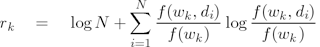
(3),
where f(wk, di) is the frequency of occurrence of
term wk
in document ti
and N is the number of
documents in the collection. The advantage of
redundancy over inverse document frequency is that it
does not simply count the documents that a type
occurs in, but takes into account the frequencies of
occurrence in each of the documents. Since it was
observed in previous work [
LK02
] that redundancy is
more effective than inverse document frequency, two
experimental settings are considered in this paper:
term frequencies f(wk,di) are multiplied by rk
as
defined in equation ( 3 ) (denoted by “+” at column
“red” in subsequent tables); or term frequencies are
left as they are: rk
≡ 1 (denoted by “-” ). For
subsequent classification an audio-visual document di
is represented by fi
or li
according to the parameter
settings.
A Support Vector Machine (SVM) is a supervised learning algorithm that has been successful in proving itself an efficient and accurate text classification technique [ Joa98, DPHS98, DWV99, LK02 ]. Like other supervised machine learning algorithms, an SVM works in two steps. In the first step — the training step — it learns a decision boundary in input space from preclassified training data. In the second step — the classification step — it classifies input vectors according to the previously learned decision boundary. A single support vector machine can only separate two classes — a positive class (y = +1) and a negative class (y = -1).
Figure 2. Operating mode of a Support Vector Machine. The SVM algorithm seeks to maximise the margin around a hyperplane that separates a positive class (marked by circles) from a negative class (marked by squares).
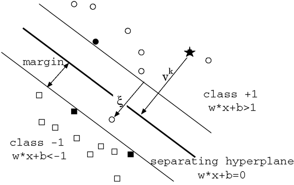
In the training step the following problem is
solved: Given is a set of training examples
Sl = {(x1,y1),(x2,y2),...,(xl,yl)}
of
size l from a fixed but unknown distribution p(x,y)
describing the learning task. The term-frequency
vectors xi
represent documents and yi
∈ {-1,+1}
indicates whether a document has been labeled with
the positive class or not. The SVM aims to find a
decision rule
h
 : x → {-1,+1}
that classifies documents as accurately as possible
based on the training set Sl
.
: x → {-1,+1}
that classifies documents as accurately as possible
based on the training set Sl
.
The hypothesis space is given by the functions f(x) = sgn(wx + b) where w and b are parameters that are learned in the training step and which determine the class separating hyperplane. Computing this hyperplane is equivalent to solving the following optimization problem [ Vap98 ], [ Joa02 ]:
minimize: 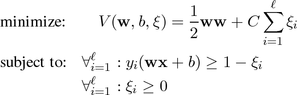
subject to:
The constraints require that all training examples are classified correctly, allowing for some outliers symbolized by the slack variables ξ i . If a training example lies on the wrong side of the hyperplane, the corresponding ξ i is greater than 0. The factor C is a parameter that allows for trading off training error against model complexity. In the limit C → ∞ no training error is allowed. This setting is called hard margin SVM. A classifier with finite C is also called a soft margin Support Vector Machine. Instead of solving the above optimization problem directly, it is easier to solve the following dual optimisation problem [ Vap98, Joa02 ]:
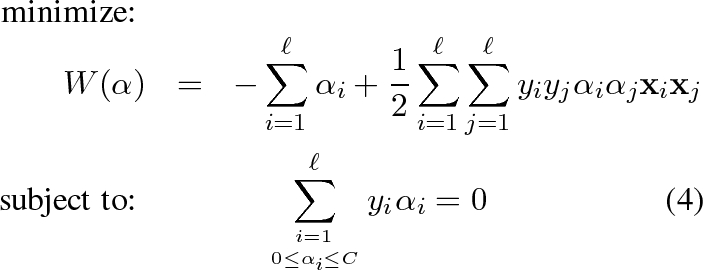
All training examples with α i > 0 at the solution are called support vectors. The Support vectors are situated right at the margin (see the solid circle and squares in figure 2 ) and define the hyperplane. The definition of a hyperplane by the support vectors is especially advantageous in high dimensional feature spaces because a comparatively small number of parameters — the αs in the sum of equation ( 4 ) — is required.
In the classification step an unlabeled term-frequency
vector is estimated to belong to the class
ŷ = sgn (wx + b)
(5)
Heuristically the estimated class membership ŷ corresponds to whether x belongs on the lower or upper side of the decision hyperplane. Thus estimating the class membership by equation ( 5 ) consists of a loss of information since only the algebraic sign of the right-hand term is evaluated. However the value of v = wx + b is a real number and can be used for voting agents, i.e. a separate SVM is trained for each modality resulting in three values vspeech ,vvideo and vaudio . Instead of calculating equation ( 5 ) we calculate ŷ = sgn(g(vspeech ,vvideo ,vaudio )) where g(∙) is the sum or the maximum or another monotone function of its arguments. We have experimented with different settings of this kind but with little success.
It is well known that the choice of the kernel function is crucial to the efficiency of support vector machines. Therefore the data transformations described above were combined with the following different kernel functions:
- Linear kernel (L):
K(xi,xj) = xi∙xj - 2nd and 3rd order polynomial kernel (P(d)):
K(xi,xj) = (xi∙xj)d d=2, 3 - Gaussian rbf-kernel (R(&gamma)):
K(xi,xj)=e-γ||xi-xj|| γ=0.2, 1, 5 - Sigmoidal kernel (S):
K(xi,xj) = tanh(xi∙xj)
In some of the experiments these kernel functions
were combined to form composite kernels, which use
different kernel functions for each modality (for
example L for speech, R(1) for video and P(3) for
audio). Formally a composite kernel is defined as
follows: Let the input space consist of Ls
speech
attributes, Lv
video attributes, and La
audio attributes,
which are ordered in such a way, that dimension 1 to
Ls
correspond to speech attributes, dimensionsLs
+1 correspond to Ls
+ Lv
video attributes, and
dimensionsLs
+ Lv
+1 to Ls
+ Lv
+ La
correspond
to audio attributes. Let  be the projection from
the input space to its subspace spanned by dimensions
k to l. A composite kernel that uses kernel K1
for
speech, K2
for video and K3
for audio is defined
as
be the projection from
the input space to its subspace spanned by dimensions
k to l. A composite kernel that uses kernel K1
for
speech, K2
for video and K3
for audio is defined
as
We think that this negative result is interesting, because the fact that the different modalities speech, video and non-speech audio do not require different treatment suggests that the respective semiotic systems are not as independent as it is often supposed.
We use a soft margin Support Vector Machine with
assymetric classification cost in a 1-vs-n setting, i.e.
for each class an SVM was trained that separates this
class against all other classes in the corpus. The cost
factor by which the training errors on positive
examples outweigh errors on negative examples is set
to  , where #pos and #neg are the number
of positive and negative examples respectively. This
means that the weight of false positive training
errors is larger for smaller classes, and in the case
#neg = #pos positive examples on the wrong side of
the margin are given twice the weight of negative
examples. The trade-off between training error and
margin was set to
, where #pos and #neg are the number
of positive and negative examples respectively. This
means that the weight of false positive training
errors is larger for smaller classes, and in the case
#neg = #pos positive examples on the wrong side of
the margin are given twice the weight of negative
examples. The trade-off between training error and
margin was set to  which is
the default in the SVM implementation that we
used.
which is
the default in the SVM implementation that we
used.
It is well known that the choice of kernel functions is crucial to the efficiency of support vector machines. Therefore the data transformations described above were combined with the homogeneous kernel functions defined in equation ( 6 ).
The following tables show the classification results
on the basis of the different modalities. A “+” in the
column “red.” indicates that the importance-weight
redundancy is used, and “-” indicates that no importance
weight is used. The values of the significance
threshold θ (used exclusively for syllables in speech
experiments) are θ = 0.1 and θ = 1. The column
“transf.” indicates the frequency transformation that
was used, “log” stands for logarithmic frequencies
with L2
-normalization and “rel” means relative
frequencies (i. e. frequencies with L1
-normalization).
The next column “kernel” indicates the kernel
function: L is the linear kernel, S is a sigmoidal
kernel, and P(d) and R(γ) denote the polynomial
kernel and the rbf-kernel respectively. The last column
shows the classification result in terms of the F-score,
which is calculated as
![]() where rec and prec are the usual definitions of
recall and precision [
MS99
]. Since a 1-to-n scheme
was used for classification the results of classifying
each class against all other classes are presented in
individual rows. All classification results presented in
this section were obtained by tenfold crossvalidation,
where the vocabulary is held constant. This makes
the results statistically reliable. Crossvalidation
involving vocabulary generation is unnecessary
because the data set used for the generation of
the vocabulary is separate from the multimedia
corpus.
where rec and prec are the usual definitions of
recall and precision [
MS99
]. Since a 1-to-n scheme
was used for classification the results of classifying
each class against all other classes are presented in
individual rows. All classification results presented in
this section were obtained by tenfold crossvalidation,
where the vocabulary is held constant. This makes
the results statistically reliable. Crossvalidation
involving vocabulary generation is unnecessary
because the data set used for the generation of
the vocabulary is separate from the multimedia
corpus.
Note that a correlation matrix between features from different modalities cannot be presented in a meaningful way. Each of the three modalities is represented by more than 1000 features (see table 2 , 3 and 4 ) and this is would lead to a correlation matrix with more than 109 entries.
The results on speech-based classification for the optimal combinations of parameters are presented in in table 5 . From the speech recognizer output syllable-n-grams were constructed for n = 1 to n = 6. Most classes were best classified with rbf-kernels (cf. table 5 ).
Table 5. Results of the classification on the basis of syllable sequences.
|
Results based on speech |
||||||
|
category |
n |
red. |
θ |
transf. |
kernel |
F-score |
|
justice |
1 |
+ |
1.00 |
rel |
R(1) |
65.0 |
|
economy |
2 |
+ |
1.00 |
rel |
P(2) |
59.3 |
|
labour |
1 |
+ |
1.00 |
rel |
R(1) |
85.3 |
|
politics |
2 |
+ |
1.00 |
rel |
R(0.2) |
74.7 |
|
sport |
1 |
+ |
1.00 |
rel |
R(5) |
80.3 |
|
conflicts |
2 |
+ |
1.00 |
rel |
R(0.2) |
73.5 |
|
advertis. |
1 |
- |
1.00 |
log |
R(0.2) |
85.0 |
Note that only sequences of one or two syllables were used for classification. This replicates an earlier result [ PLL02 ]: The optimal unit-size for spoken document classification is often smaller than a word (in German the average word length is ~ 2.8 syllables) especially under noisy conditions.
Table 6 shows results based on a vocabulary of 100 video signs, table 7 those for 400 video signs. The length of the video words (i.e. the length of the n-gram) is given in column 2 and the accuracy is presented in column 6. In the case of a visual lexicon of 100 video signs the units used for classification are n-grams with a size varying from n = 1 to n = 5. This means that these units are built using one to five video-shots. Those categories that are classified on the basis of shot-unigrams show relatively poor accuracy.
Table 6. Classification results based on a visual vocabulary of 100 video signs
|
F-scores obtained using small visual vocabulary |
|||||
|
category |
n |
red. |
transf. |
kernel |
F-score |
|
justice |
4 |
- |
log |
S |
46.4 |
|
economy |
3 |
- |
rel |
R(5) |
29.1 |
|
labour |
2 |
- |
log |
S |
41.6 |
|
politics |
4 |
- |
rel |
R(1.0) |
48.5 |
|
sport |
5 |
+ |
rel |
R(0.2) |
51.9 |
|
conflicts |
2 |
- |
log |
R(0.2) |
35.0 |
|
advertis. |
1 |
- |
log |
R(1) |
85.7 |
We therefore believe that we have detected regularities in the succession of video-units, which reveal a kind of temporal (as opposed to spatial) video-syntax. Rbf-kernels seem to be the most appropriate for classification on the basis of video-words when a small set of video signs is considered.
Table 7. Classification results based on a visual vocabulary of 400 video signs
|
F-scores obtained using large visual vocabulary |
|||||
|
category |
n |
red. |
transf. |
kernel |
F-score |
|
justice |
1 |
- |
log |
S |
42.0 |
|
economy |
1 |
+ |
log |
L |
31.2 |
|
labour |
3 |
- |
log |
S |
31.2 |
|
politics |
2 |
- |
rel |
S |
53.4 |
|
sport |
4 |
+ |
rel |
R(5) |
53.8 |
|
conflicts |
1 |
- |
rel |
L |
39.8 |
|
advertis. |
5 |
+ |
rel |
R(1) |
91.2 |
With more video signs to choose from, the performance increases significantly (with the exception of the categories “labour” and “justice”), and the n-gram length decreases.
We attribute this to the fact that the semantic specificity ofn-grams increases with n. As units from a larger vocabulary are on average semantically more specific than units from a smaller one, the specificity of video-words obtained from the larger vocabulary is compensated by a decrease of n-gram degree. Results for optimal parameter settings and different sizes of the visual vocabulary are presented in figure 3 . Vocabularies of 400 video signs yielded the best results on average. This vocabulary size is also used for integration of modalities described in section 5.4 .
Figure 3. Classification performance vs. vocabulary size. Different classes show different behaviour when the vocabulary size is changed. A vocabulary size of 400 video signs seems to be optimal. Note that the visual vocabulary which was obtained from the test corpus itself (labeled as “corpus”) does not yield better classification results compared to the others.
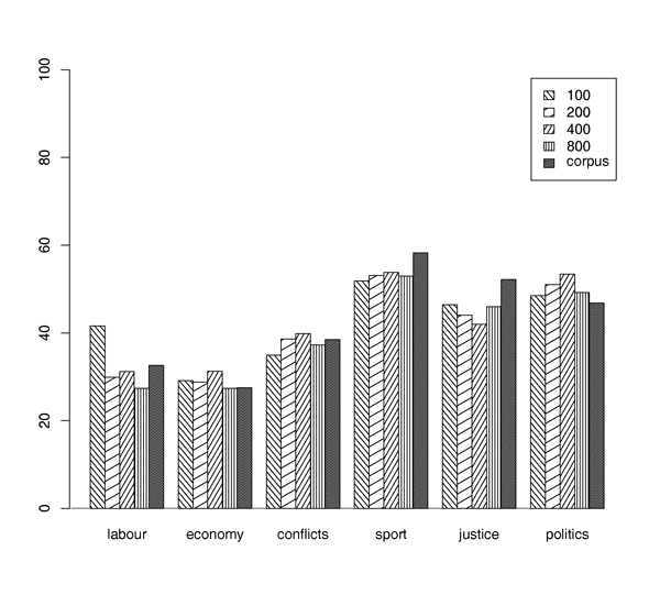
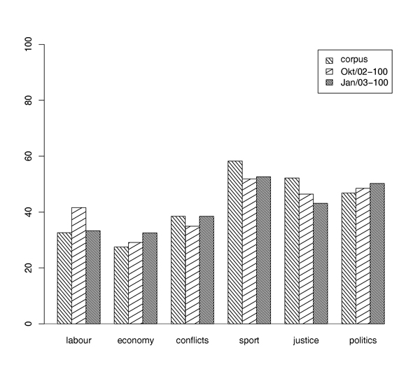
One might argue that the collection of a visual vocabulary at a point in time different from the test corpus is flawed because typical images cannot be present in both corpora. However our principal assumption was that the video words reveal a kind of implicit code, which is known to the individuals of a given society. The assumption of the existence of such a code implies that it is shared by the members of the society and functions as a means to convey (non-linguistic) information. To fulfil this communicative function a code may not vary too quickly and should apply to past and future alike. As can be seen in figure 4 , experimental results with visual lexicons created at different times (summer 2002 and January 2003) did not show a consistent change in performance and support the assumption that the vocabulary is independent from the acquisition date. For the practical application this means that once a visual vocabulary is generated it can be used for a long period of time.
From figure 4 one can see that the effect of the change of the visual semiotic system is limited. This is reflected in the results of the classification. Categories “justice” and “sports” and to a lesser extent “politics” show a decrease of performance when the lexicon was drawn from the October material instead of the corpus itself. This can be attributed to the fact that there were salient news in these categories at the time when the corpus was sampled, namely the soccer world championship (sports) and a massacre at a German high school (justice).
The results for the categories “economy” and “conflicts” are nearly independent from the creation date of the visual lexicon. These categories are communicated by visual signs that seem to be temporarily invariant.
The relatively good results for video classification suggest that the task of supervised content classification of audio-visual news stories is different form the recognition of objects on images for retrieval purposes. News stories are not pictures of reality. They are man-made messages intended to be received by the news observers. Thus the regularities between content and visual expression follow aesthetical rules rather than reality itself.
In his semiotic analysis of images Roland Barthes distinguishes between the denoted message and a connoted message of a picture. In his view all imitative arts (drawings, paintings, cinema, theater) comprise two messages: a denoted message, which is the analogon itself, and a connoted message, which is the manner in which the society to a certain extent communicates what it thinks of it. The denoted message of an image is an analogical representation (a ′copy′) of what is represented. For instance the denoted message of an image which shows a person is the person itself. Therefore the denoted message of an image is not based on a true system of signs. It can be considered as a message without a code. The connotive code of a picture in contrast results from the historical or cultural experience of a communicating society. The code of the connoted system is constituted by a universal symbolic order and by a stock of stereotypes (schemes, colors, graphisms, gestures. expressions, arrangements of elements). [ Bar88 ]
The rationale behind the use of low-level video features is not to discover the denoted message of a video-artefact (whether it shows for instance a person or a car) but to reveal the implicit code which underlies its connoted message. We suppose that some of the aspects of the connoted code postulated by Barthes are reflected in the video words.
Figure 4. Classification performance vs. date of vocabulary acquisition. The visual vocabularies were generated from different training corpora which were sampled at different instances of time: January 2003, October 2002 and April to June 2002, denoted as “corpus”. The figure shows that the variation between classes is larger than the variation between different lexicon creation times.
Classification on the basis of non-speech audio words is shown in table 8 . The error rates are worse than those of the other two modalities (speech and video). The only category which is accurately classified is “advertisement”. Most classifications are based on audio sign unigrams, i.e. audio words that consist of only one audio sign. Building sequences of audio signs generally does not improve the performance. This means that, in contrast to video words, the audio words do not represent a kind of temporal syntax.
Table 8. Comparison of results for non-speech audio with different audio signs and different sizes of non-speech audio vocabularies.
|
F-scores obtained using different sizes of non-speech audio vocabulary |
|||||||||
|
|
50 signs |
100 signs |
200 signs |
||||||
|
|
4 frames |
8 frames |
16 frames |
4 frames |
8 frames |
16 frames |
4 frames |
8 frames |
16 frames |
|
justice |
35.4 |
34.6 |
35.2 |
36.0 |
35.4 |
37.3 |
36.9 |
36.1 |
35.5 |
|
economy |
21.1 |
22.5 |
22.8 |
23.9 |
23.5 |
20.6 |
20.1 |
24.0 |
24.5 |
|
labour |
18.9 |
17.0 |
20.6 |
21.8 |
16.8 |
18.6 |
19.6 |
18.2 |
19.6 |
|
politics |
47.0 |
46.9 |
46.1 |
48.6 |
47.3 |
46.6 |
45.7 |
46.7 |
44.9 |
|
sport |
40.8 |
32.2 |
35.3 |
38.2 |
31.4 |
39.0 |
35.1 |
35.3 |
36.0 |
|
conflicts |
27.8 |
24.5 |
28.9 |
28.2 |
22.1 |
28.9 |
27.2 |
23.6 |
25.6 |
|
advertis. |
90.5 |
90.4 |
91.2 |
92.1 |
93.3 |
90.2 |
93.2 |
92.4 |
91.8 |
In contrast to video there is no dependency between size of vocabulary and length of n-grams that form audio words. We thus conclude that, in contrast to the video words, the audio words do not reveal an implicit acoustic code. There is also no clear pattern of a relationship between the number of frames that form the audio signs and vocabulary size as can be seen from table 8 . However, audio signs based on 4 frames yield slightly better results than the other frame lengths. The best results in average were obtained for a vocabulary of 100 audio signs based on a 4-frame audio features. From exploratory experiments we decided to use a vocabulary of 50 audio signs based on 4 frames for the integration with the other media. Although non-speech audio yielded poor results as a single modality, it is beneficial when combined with speech.
Figure 9 directly compares the error rates of all single modalities. There is a clear ranking among the three modalities, when they are employed individually. Speech yields best results for most classes, and video is by far better than non-speech audio. There is however one exception to the disappointing results of non-speech audio. The generally superb rates of the category “advertisement” are likely to be caused by the shot duration in commercial spots, which is generally very short. Furthermore the audio in advertisements is usually compressed causing the overall energy in the audio spectrum to be considerably higher than normal, which is reflected by the audio-features that we used. Another aspect is that commercials are broadcast repeatedly. Therefore in some cases identical spots are present in both test and training data.
Table 9. Comparison of the results on single modalities, that were obtained with optimal parameter-settings
|
Largest F-scores vs. chance |
||||
|
category |
speech |
video |
audio |
chance |
|
justice |
65.0 |
42.0 |
36.0 |
17.3 |
|
economy |
59.3 |
31.2 |
23.9 |
9.8 |
|
labour |
85.3 |
31.2 |
21.8 |
7.0 |
|
politics |
74.7 |
53.4 |
48.6 |
28.9 |
|
sport |
80.3 |
53.8 |
38.2 |
13.0 |
|
conflicts |
73.5 |
39.8 |
28.2 |
12.3 |
|
advertis. |
85.0 |
91.2 |
92.1 |
17.1 |
From exploratory experiments we concluded that proper adjustment of the vocabulary sizes of the different modalities is crucial to a successful integration of modalities. A visual vocabulary of 400 audio signs and a acoustical vocabulary of 50 audio signs calculated on the basis of 4 frames turned out to be optimal when integrating two or three modalities.
Table 10 shows results of the combined modalities non-speech audio and video. The F-scores are better than those based exclusively on non-speech audio, but not better than those of single video (see table 9 and 7 ) and still much worse than a combination of speech with non-speech audio or video. We conclude that the combination of video and non-speech audio generally does not improve classification.
Table 10. Results of the classification with both audio-words and video-words.
|
F-scores obtained using video and non-speech audio |
||||||
|
category |
n(audio) |
n(video) |
red. |
transf. |
kernel |
F |
|
justice |
1 |
5 |
+ |
rel |
S |
42.0 |
|
economy |
1 |
1 |
- |
log |
R(0.2) |
30.1 |
|
labour |
3 |
3 |
- |
log |
S |
29.8 |
|
politics |
1 |
1 |
+ |
log |
R(0.2) |
51.7 |
|
sport |
1 |
3 |
- |
rel |
R(0.2) |
51.0 |
|
conflicts |
5 |
1 |
- |
rel |
R(5) |
38.3 |
|
advertis. |
5 |
3 |
+ |
log |
S |
93.9 |
The picture changes when video is combined with speech. Especially the classes “advertisements” and “sports” show an improvement over the single modalities for the combination of video and speech (see table 11 ). Interestingly the optimal parameters have changed: sigmoidal and linear kernels perform best for all classes — a phenomenon that extends to the integration of all modalities — and the lengths of video words and syllable-n-grams is slightly changed compared to the single modalities (see tables 5 and 7 ). The combination of speech and video is especially advantageous for the category “sport”, but adding non-speech audio yields a further improvement of accuracy (see table 13 ).
Table 11. Results of the classification with both n-grams of video signs and syllable n-grams.
|
F-scores obtained using video and speech |
|||||||
|
category |
n |
n |
red. |
θ |
transf. |
kernel |
F |
|
justice |
1 |
1 |
+ |
1.00 |
log |
L |
67.3 |
|
economy |
2 |
2 |
+ |
1.00 |
log |
S |
55.1 |
|
labour |
2 |
2 |
+ |
1.00 |
log |
S |
84.8 |
|
politics |
1 |
2 |
- |
1.00 |
log |
L |
70.7 |
|
sport |
3 |
2 |
+ |
1.00 |
log |
S |
86.2 |
|
conflicts |
2 |
2 |
+ |
1.00 |
log |
S |
67.9 |
|
advertis. |
3 |
1 |
+ |
1.00 |
log |
S |
93.4 |
Table 12 shows the results of the combined modalities speech and non-speech audio. The accuracy of all classes (with the exception of “justice” and “politics”) improves when non-speech audio is added to speech (see table 5 and 9 ). The categories “conflicts” and “economy” can best be classified with the combination of speech and non-speech audio.
The result on the combination of speech and non-speech audio has an implication to speech classification in general: It can be useful to base speech classification not solely on linguistically defined features. Especially when the speech data was sampled under realistic conditions and contains background noise and other non-speech signals. Results on fenone recognition point in the same direction [ Har01 ]. Fenone-based classification works even when the signal is so noisy that it cannot be understood by a human listener.
One difference between the combination of speech and non-speech audio and the combination of speech and video is that optimal n-grams for both syllables and audio-signs are in most cases longer than those of the single modalities. In the case of the category “justice” syllable n-grams and audio words are used up to the maximal length (n = 6). In other words, all available information is used, but the classifier cannot find a hyperplane that is consistent with the patterns of both speech and non-speech audio. A different kernel function or an adjustment of the speech and non-speech subspace of the input space might have improved the situation.
Table 12. Results of the classification with both n-grams of non-speech audio and syllable n-grams
|
F-scores using speech and non-speech audio |
|||||||
|
category |
n |
n |
red. |
θ |
transf. |
kernel |
F |
|
justice |
6 |
6 |
+ |
0.1 |
rel |
R(1) |
63.3 |
|
economy |
1 |
5 |
+ |
1.0 |
rel |
R(5) |
62.7 |
|
labour |
5 |
4 |
+ |
1.0 |
rel |
R(5) |
89.6 |
|
politics |
6 |
2 |
+ |
1.0 |
rel |
R(0.2) |
72.5 |
|
sport |
2 |
2 |
+ |
1.0 |
log |
S |
83.5 |
|
conflicts |
1 |
2 |
+ |
1.0 |
log |
S |
74.1 |
|
advertis. |
1 |
2 |
+ |
0.1 |
log |
S |
92.0 |
Table 13 shows results of all combined modalities. The category “labour” benefits most from the integration of modalities. The combination of the modalities speech and non-speech audio leads to improved accuracy compared to speech alone. Adding video yields even better results for the classes “sport”, “labour” and “advertisement”. The F-scores of “labour”, “sport”, “conflicts”, and “advertisement” are better than those of the single speech modalities (see table 9 ). The reason seems to be that these categories show many explicit non-speech features which make them distinguishable from others. This does not seem to be the case for other categories like politics, where pictures and sounds are not as important as words. In this last table we have added the F-scores based on classification by chance. These scores are independent of the modalities used for classification and can also be compared to all other F-scores in the previous tables.
Table 13. Results of the classification with audio-words (50 signs, 4 frames), video-words (400 signs) and sequences of syllables, compared to the F-measure according to chance. The choice of parameters was restricted to sigmoidal kernels, logarithmic frequencies and the application of term weighting according to equation ( 3 ).
|
F-scores obtained using speech, video, and audio |
|||||
|
category |
n(audio) |
n(speech) |
n(video) |
F |
chance |
|
justice |
4 |
5 |
3 |
62.1 |
17.3 |
|
economy |
5 |
3 |
2 |
58.8 |
9.8 |
|
labour |
4 |
2 |
4 |
91.4 |
7.0 |
|
politics |
3 |
3 |
3 |
72.6 |
28.9 |
|
sport |
4 |
4 |
2 |
87.2 |
13.0 |
|
conflicts |
4 |
4 |
1 |
73.0 |
12.3 |
|
advertis. |
2 |
1 |
5 |
94.6 |
17.1 |
The optimal combination of modalities depends very much on the content class. There is no combination of modalities that yields good results for all classes. Media integration was unsuccessful for the category “politics”, which was best classified (F=74.7) on the basis of syllable bigrams. The category “justice” is best classified with video and speech: F=67.3. The category “conflicts” is best classified with speech and non-speech audio (F=74.1), and so is “economy” (F=62.7). The categories, “sport” (F=87.2), “labour” (F=91.4) and “advertisement” (F=94.6) are best classified with all three modalities.
Audio and video words constructed from low-level features provide a good basis for the integration of modalities in order to classify audio-visual documents. Homogeneous kernels (see section 4.2 ) are a good solution to the integration of modalities. The optimal combination of modalities depends, however, on the category to be recognized. This is an important result, since multimodal analysis and retrieval algorithms exploiting the synergy between the various media are currently considered as one of the major challenges of future research in multimedia information retrieval [ LSDJ06 ].
The visual vocabularies generated as described in this paper are to a certain extent temporally stable. This allows to create a visual lexicon before the actual video classification is performed. The classification performance based on video alone depends on the lexicon size. As units from a larger vocabulary are on average semantically more specific than units from a smaller one, the specificity of video-words obtained from the larger vocabulary is compensated by shorter video words.
Classification based on speech outperforms all other single modalities. Combining speech with non-speech audio improves classification. Classification is further improved by supplementing speech and non-speech audio with video words. Optimal F-scores range between 62% and 94% corresponding to 50% - 84% above chance.
The results, that were obtained exclusively on non-speech audio, are disappointing. Furthermore the classification on non-speech audio does not benefit from higher order n-grams. This suggests that there are no regularities in the temporal combination of audio units at any of the timescales that we have considered.
We therefore think that the audio features, that we exploited (spectrum flatness and spectrum envelope) were not useful for our approach. The classification performance based on non-speech audio may improve when different low-level features are used for the generation of audio words. Future research will deal with the improvement of non-speech audio features.
Although non-speech audio words yield poor results as a single modality they are beneficial when combined with syllable n-grams. This suggests that it can be useful to base speech classification not solely on linguistically defined features. Especially when the speech data was sampled under realistic conditions and contains background noise and other non-speech signals, non-speech audio seems to be beneficial.
The major disadvantage of our approach is the need for a semantically annotated corpus of AV-scenes. Its major strength, however, is that it yields a high-level semantic description of AV-documents. The generation of the visual and non-speech audio vocabularies requires a lot of effort as well as the training of the SVMs. The vocabularies however can be used for a long period time as figure 4 suggests, and we suppose that this also holds for trained SVMs. Training the classifier and generation of the vocabularies can therefore be done off-line from time to time. The training phase, however, is fast. Our method yields a high-level semantic description at low cost in the classification phase, and this is its benefit compaired to conventional techniques that use audio and visual information directly from the news stream.
Our Approach can be used to represent the AV-documents in a semantic space. To this end modify the classification step of the SVM and interpret the valuev = wx + b in equation 5 as a vote for the respective class. This generates a semantic space whose dimensions correspond to the degree of membership to each of the classes that have previously been learned. Such a construction of a semantic space yields a semantically transparent description of the multimodal documents in contrast to other techniques like (probabilistic) latent semantic analysis.[ LMP04, Leo05 ]
Future research will deal with the possibility to learn a classifier on one modality in order to classify another. This has successfully been done with written and spoken documents [ PLL02 ] and we suppose that it can also be applied to speech, video and non-speech audio. The procedure is as follows: train a classifier on speech, classify AV-documents using this classifier. The result is a corpus of semantically annotated AV-documents that can be used in order to train a classifier for video or non-speech audio. Large corpora of semantically annotated written texts are available from the news agencies. They could be used in order to generate a training corpus for multimedia classification.
This study is part of the project Pi-AVIda which is funded by the German ministry for research and technology (BMFT) (proj. nr. 107). We thank the Institute for Communication and Phonetics of the University of Bonn for contributing the BOSSII system and Thorsten Joachims (Cornell University) who provided the SVM-implementation SVMlight. Furthermore we thank Fraunhofer Institutes IMK, IGD and IIS for the extration of the speech, video and non-speech audio data. We also thank our collegues Gerhard Paaß and Hugo de Vries for fruitful discussions.
[Bar88] Image - Music - Text: Essays, Noonday Press, New York, 1988, isbn 0-374-52136-0.
[CLL99] Automatic harmonic description of musical signals using schema-based chord decomposition, Journal of New Music Research 1999, no. 4, 310—333 issn 0920-8215.
[DPHS98] Inductive learning algorithms and representations for text categorization , Proceedings of the seventh International Conference on Information and Knowledge Management CIKM'98, pp. 148—155, ACM Press, New York, 1998, isbn 1-58113-061-9.
[DWV99] Support vector machines for spam categorization, IEEE Transactions on Neural Networks (1999), no. 5, 1048—1054, issn 1045-9227.
[FGJ95] In search of a simple visual vocabulary , Proceedings of the 11th ieee International Symposium on Visual Languages vl'95, pp. 302—309, ACM Press, Darmstadt, Germany, 1995, isbn 0-8186-7045-2.
[FGL04] Multi-level annotation of natural scenes using dominant image components and semantic concepts , Proceedings of the ACM International Conference on Multimedia, pp. 540—547 ACM Press, New York, 2004, isbn 1-58113-893-8.
[Har01] Automatische Verfahren zur Sprachdetektion, Landessprachenerkennung und Themendetektion, Berlin, Logos, 2001, isbn 3-89722-766-5.
[Hug75] , Temporally Segmented Speech, Perception & Psychophysics (1975), no. 2, 149—157, issn 0031-5117.
[Joa98] Text categorization with support vector machines: learning with many relevant features, Proceedings of the 10th European Conference on Machine Learning ecml'98, Lecture Notes in Computer Science, Vol. 1398, Chemnitz, Germany, 1998, pp. 137—142, isbn 3-540-64417-2.
[Joa02] Learning to Classify Text using Support Vector Machines , Kluwer Academic Publishers, Boston, 2002, isbn 0-7923-7679-X.
[Leo02] Artificial Semiotics, pp. 659—670, Winfried Nöth and Guido Ipsen (Eds.), Körper - Verkörperung - Entkörperung. Proceedings of the 10th Internationalen Congress of the German Association for Semiotic Studies (dgs), 2002, Kassel University Press, isbn 3-89958-045-1.
[Leo05] , On semantic spaces, ldv-Forum (2005), no. 1, 63—86, issn 0175-1336.
[LEP02] Exploring subword features and linear Support Vector Machines for German Spoken Document Classification, Proceedings of the International Conference of Spoken Language Processing icslp'02, 2002, pp. 2989—1992 .
[Lew00] Next Generation Web Searches for Visual Content, IEEE Computer November (2000), 46—53, issn 0018-9162.
[LK02]
Text Categorization with Support Vector Machines. How to Represent Texts in Input Space?,
[LMP04] Data Mining and Text Mining for Science & Technology Research, Handbook of Quantitative Science and Technology Research, Henk F. Moed, Wolfgang Glänzel, and Ulrich Schmoch(Eds.), Kluwer Academic Publishers, Dordrecht, Boston, London, 2004, pp. 187—214, isbn 1-4020-2702-8.
[LSDJ06] Content-based Multimedia Information Retrieval. State of the Art and Challenges, ACM-Transactions of Multimedia Computing, Communications, and Applications (2006), no. 1, 1—19, issn 1551-6857.
[LW03] Automatic Linguistic Indexing of Pictures by a Statistical Modeling Approach, ieee Transactions on Pattern Analysis and Machine Intelligence (2003), no. 9, 1075—1088, issn 0162-8828.
[MS99] Foundations of Statistical Natural Language Processing, MIT Press, Cambridge, 1999, isbn 0-262-13360-1.
[PLL02] SVM Classification Using Sequences of Phonemes and Syllable, Proceedings of the 6th European Conference on Principles of Data Mining and Knowledge Discovery PKDD 2002, Springer, 2002, Lecture Notes in Computer Science , pp. 373—384, isbn 3-540-44037-2.
[Poe85] Grenzen des Bewußtseins: Über Wirklichkeit und Welterfahrung , Deutsche Verlagsanstalt, Stuttgart, Germany, 1985, isbn 3-421-02735-8.
[RPW06] Handbuch Visuelle Mediengestaltung , Cornelsen, Berlin, 2006, isbn 3-589-23655-8.
[RSP03] Detecting Semantic Concepts from Video Using Temporal Gradients and Audio Classification, Proceedings of the 3rd International Conference on Image and Video Retrieval, Urbana, Springer, Berlin, 2003, pp. 260—270, isbn 3-540-40634-4.
[SWH00] Speech Synthesis by Multilevel Selection and Concatenation of Units from Large Speech Corpora, Verbmobil: Foundations of Speech-to-Speech Translation, Symbolic Computation, Wolfgang Wahlster (Ed.), Springer, 2000, pp. 519—538, New York, isbn 3-540-67783-6.
[TG99] Improved Speaker Segmentation and Segments Clustering using the Bayesian Information Criterion , Proceedings of the sixth European Conference on Speech Communication and Technology Eurospeech'99, 1999, Budapest, Hungary , isca Archive http://www.isca-speech.org/archive/euro-speech\_1999.
[Vap98] Statistical Learning Theory , Wiley & Sons, 1998, New York, isbn 0-471-03003-1.
[Vol02] Fast Approximate Nearest-Neighbor Queries in Metric Feature Spaces by Buoy Indexing , 36-49 Proceedings of the 5th International Conference on Visual Information Systems visual 2002, 2002, Springer, Hsin Chu, Taiwan, Lecture Notes in Computer Science , isbn 3-540-43358-9.
[WKMG98] Incorporating information from syllable length time scales into automatic speech recognition, pp. 721—724 Proceedings of the 23rd International Conference on Acoustics, Speech and Signal Processing ICASSP′98, , 1998, Seattle, USA, Lecture Notes in Computer Science, isbn 0-7803-4428-6.